In a class project for ECE 6552: Nonlinear Systems during Spring 2016 at Georgia Tech; Pavel Komarov, Prabhudev Prakash and I explored whether we could relate tools in nonlinear analysis, optimal control and statistical learning to each other? If so, what would the common and contrasting factors between these tools be? We compared an analytically derived nonlinear controller with a reinforcement learning controller, both designed to keep an inverted pendulum from falling down on a moving cart, by applying force to the cart. We found an interesting connection between the two kinds of controllers and made some neat videos. Click through to check it all out.
The Cart Pole System

Our objective was to balance the pole in the picture above, by applying force (F) to the cart. We did not care where and how fast the cart was moving as long as the pole did not fall down i.e go horizontal. The equations alongside the figure describe the dynamics of the cart and the pole. We chose a familiar and somewhat simple nonlinear system because our objective was to compare different approaches that might be used for control.
An Analytically Derived Nonlinear Controller
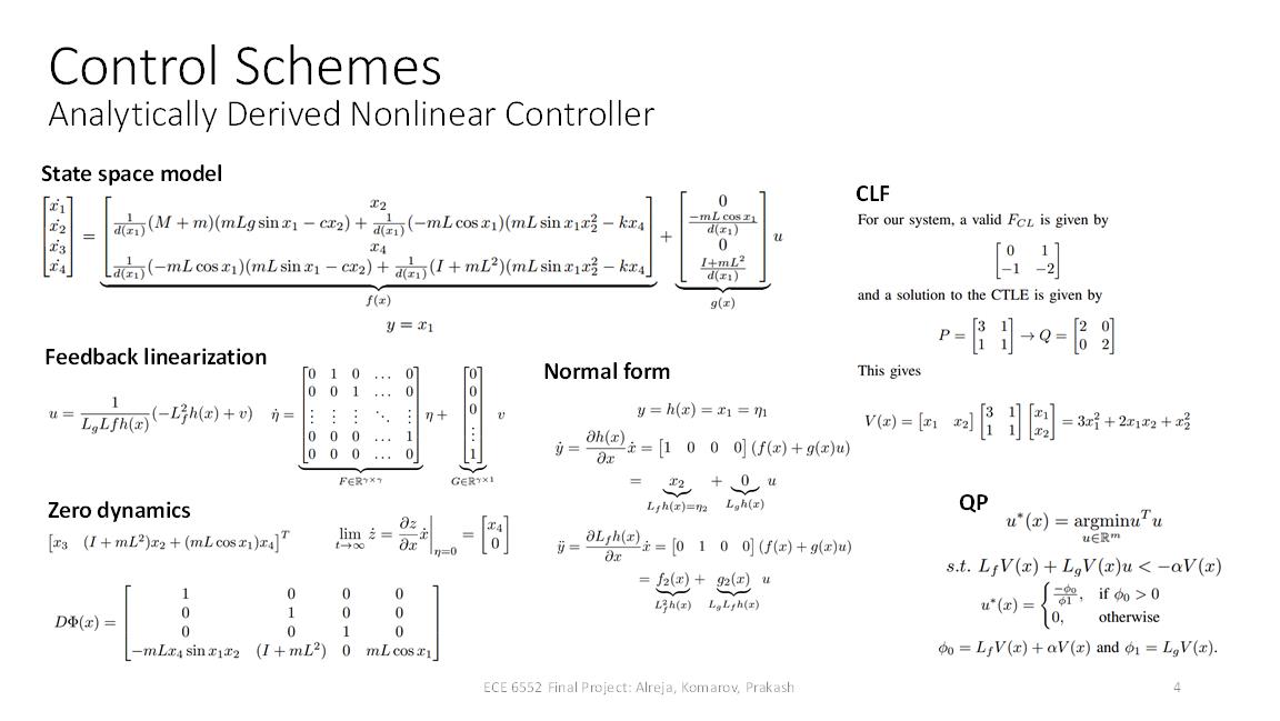
For a layperson, I will simply say we did a lot of math like the kind in the picture below. For readers who are familiar with nonlinear systems/control, we used a Control Lyapunov Function (CLF) controller whose derivation is detailed in Section III.B of our report.

Reinforcement Learning (RL) Agent as a Controller
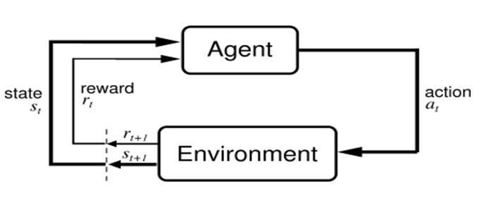
Reinforcement Learning (RL) involves an agent/controller interacting (i.e. applying a Force to the cart) with its environment (the cart-pole system) and continously receiving rewards (or punishment) $r$ for its actions in pursuit of preventing the pole from falling over. The important distinction between the RL agent and the CLF controller is that the RL agent has no idea about what the system is or the laws that govern it. Over time, the agent learns the optimal behavior (a policy $\pi$) to attain the maximum possible cumulative reward ($Q$).

The mathematical framework underlying RL is fairly abstract and vast$^{1}$. It lends itself to different implementations under different assumptions and several algorithms which instantiate the underlying mathematics behind RL (TD-Learning, SARSA, Q-Learning) exist. We used Q-learning, which involves learning the optimal action (a) for each state (s), over a finite discrete state and action space by performing stochastic gradient descent as follows.
\[Q(s,a) = Q(s,a) + \alpha\times[r+\gamma\times\max_{a'} Q(s',a')-Q(s,a)]\]Since we are dealing with a continuous system and Q-Learning operates over a finite and discrete state space, we needed to discretize the state and action space. The two variables of interest for us are the displacement ($\theta$) and the angular velocity ($\dot{\theta}$) and they are discretized as follows giving us $4\times2=8$ states

Next, we need to discretize the action space as well. We adopt a minimalistic approach, where we apply a 10 N force to the cart in the left or right direction ($F=\pm 10 N$). This means that our RL controller needs to learn the Q-values for a total of $4\times 2\times 2=16$ state-action pairs. This is a fairly coarse discretization works out pretty well in practice.
Lastly, we needed to decide how to reward or punish the Q-learning agent. We chose to give a reward of 0 at every time step where the pendulum was above the horizontal and a punishment of -1 for when it became horizontal. The pendulum falling down also reset the simulation to a randomly initialized starting position.
Q-learning can be implemented in different ways ranging from a look up table (Q-Table) to non-linear function approximators (neural networks like Deep Q Networks). We chose the simplistic Q-Table for this project because it is easy to examine and debug. Readers familiar with RL and curious about the values of various parameters that govern the algorithm’s learning may find the details in Section III.A of our report interesting.
Results
Basic Functionality of the Q-Learning Controller
The video below (credit: Prabhudev Prakash) shows how the highly simplified Q-learning controller balances the inverted pole on a cart. The red triangle depicts the direction of force application. It is clear that the pole is never perfectly upright, though it never falls down all the way. Finer discretization of the state and action space, not shown here, produces better performance in terms of accuracy and efficiency, but increases the learning time since a larger Q-Table with more parameters has to be learned. It is neat to see a simple system with 16 parameters perform such a difficult task adequately.
Basic Functionality of the analytically derived CLF controller.
The video below (credit: Pavel Komarov) shows near perfect application of force and near perfect upright position achieved by the analytically derived Nonlinear Control Lyapunov Function controller. In comparison to the RL controller, its accuracy and efficiency are striking. Not only does it smoothly solve the problem of getting the pole in an upright position, the amount of force it uses seems to converge toward 0.
Performance in Noisy conditions
In any engineered system, there is noise in our observation of the variables of interest, which never completely disappears. With this is in mind, we injected measurement noise that prevented the controllers from seeing the true state of the system accurately (details of noise injection Section IV of the report), while we as experimenters still could.

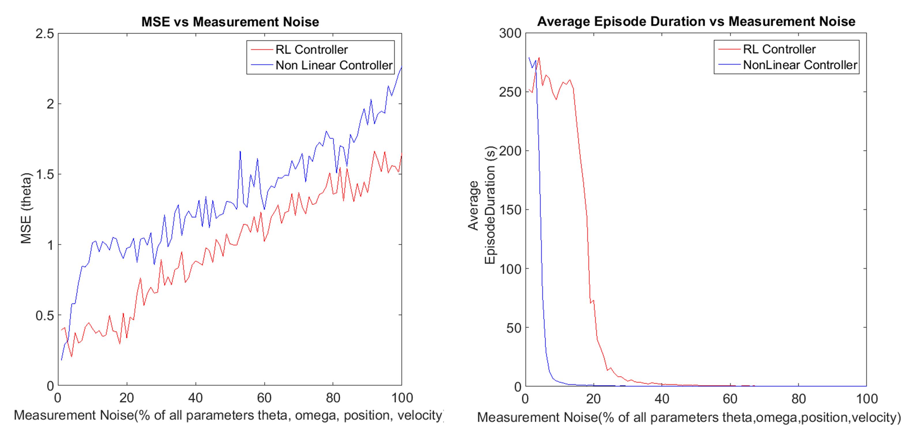
We found that the coarse grained RL controller is far more robust in the presence of noise than the fine tuned Nonlinear CLF controller. The left panel in the figure above shows that the RL controller keeps the pole relatively closer to the upright position compared to the Nonlinear CLF controller once noise is injected and the difference in performance persists as noise levels increase. The right panel in the figure above plots the duration for which each controller can last i.e. before the pole falls down/becomes horizontal as noise increases, showing that the RL controller is again more resistant to noise than the Nonlinear CLF controller.
The connection between nonlinear (CLF) and optimal learned (Q-table) controllers
Despite vast differences in the methodology, both the Q-learning and CLF controllers are doing function approximation in some form. So we decided to compare the functions they approximate/learn with each other. Here we found an interesting commonality. The Q-Function learned by our Q-table, although coarse had an eerily similar shape to the inverted CLF $V(x)$. The video below sketches these two functions out and looks at them from different angles for more convincing visual than a single figure might offer.
If this generalizes beyond our simple-system, curve-fitting a function to an RL’s Q-table could be a powerful tool to guide design CLF-based controllers for systems that resist analytical tractablility. The best part of this result for us was that it emerged from a system-agnostic reward scheme: The learner knew nothing of the natural environment aside from the fact that letting the pendulum fall was bad, yet it was able to distribute that information over the whole state-space in such a way that its notion of “goodness” for a state is related to that state’s energy. This suggests that Lyapunov Stability theory is a truth commonly reflected in nature.
Conclusion
With a simple scheme, the RL controller learns to perform the task of keeping the inverted pole (relatively) upright. The analytically derived CLF controller is far more efficient and accurate at performing the same task. However, when noise enters the system, this situation reverses. The RL controller’s design uses discretization which induces quantization noise and as a result it proves more robust in noisy conditions than the CLF controller.
This suggests that while analytically approaches are superior in domains requiring efficiency and accuracy. An RL based method may be more effective in noisy conditions. Moreover, since they require no deep analysis of system dynamics, they can be useful in domains where such analysis is not tractable.
Beyond this either-or view, we felt that these methods can be used together. Particularly for control objectives requiring stabilization to an energetically critical point, it appears that it may be possible to find a CLF by curve fitting the Q-values of an RL controller. Such an approach would not require the complicated analysis required to derive the CLF controller and might be particualrly useful in situations where such analysis is not possible. Future work along these lines might focus on whether our observations with the simple cart-pole system can generalize to higher dimensional systems which have more complex dynamics.
